Manufacturing and quality assurance processes in electronics production, mechanical engineering and the automotive industry increasingly require multi-axis positioning systems. At the same time, the requirements in terms of accuracy are also increasing.

Depending on the model, parallel-kinematic hexapod robots can move and position tools, workpieces, and complex components with weights ranging from a few grams to several hundred kilograms or even several tons in any spatial orientation with high precision – regardless of the assembly orientation.

The PI hexapod controller with integrated EtherCAT® interface now makes it very easy for users to integrate hexapods into automation systems without it being necessary to perform challenging kinematic transformations. This article details how the integration works, how Work and Tool coordinate systems can be used, and how the range of motion of the hexapod is optimally used.

Hexapods in Comparison with Serial- Kinematic Systems

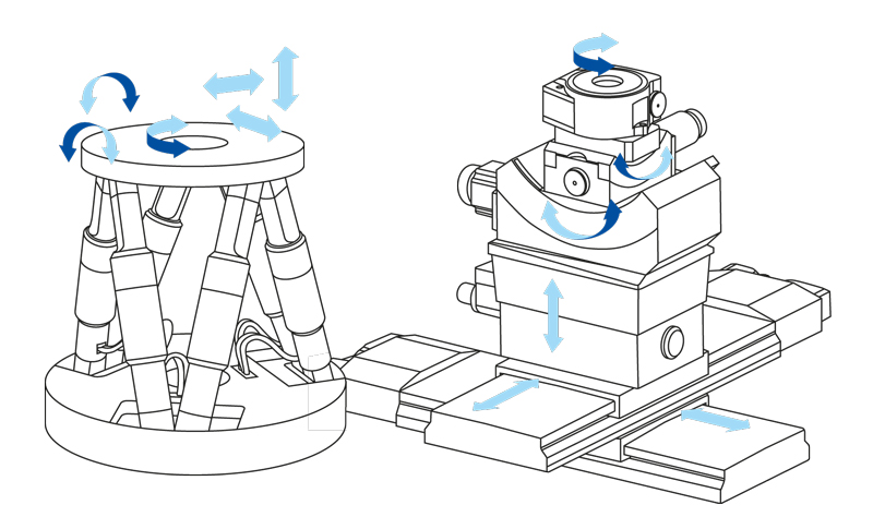
Serial-kinematic systems consist of individual axes or actuators that build on each other, which means they are mechanically connected in series. For example, a platform-bearing Z-axis is mounted on a Y-axis, which in turn is mounted on an X-axis (figure 1).

.

In hexapods, all six actuators act directly on a single platform. This allows a considerably more compact setup than is the case with serially stacked multi-axis systems.

Since only a single platform is moved, which is also often equipped with a large aperture, the mass moved is considerably lower, resulting in significantly improved dynamics.In addition, hexapods exhibit higher accuracy, since they usually do not contain guides with corresponding guide errors and the errors from the individual drives do not compound. Since the cables are not moved with the platform, the precision is not influenced by corresponding friction or torques. In addition, the parallel structure increases the stiffness and thus the natural frequencies of the overall system as well.

In stacked systems, however, the lower drives not only have to move the mass of the payload, but also the mass of the drives that follow, along with their cables. This reduces the dynamic properties. Guiding errors that accumulate on the individual axes also impair accuracy and repeatability.

Figure 1: Functional scheme of parallel-kinematic hexapods in comparison with serially stacked axes (PI).

An essential feature of the hexapods are the freely definable reference coordinate systems for the tool and workpiece position (Work, Tool). This allows the movement of the hexapod platform to be specifically adapted to the respective application and integrated into the overall process.

Simple Integration Despite Complex Kinematics: Hexapod Systems Employ Intelligent Multi-Axis Drives with Fieldbus Connection

In a parallel-kinematic system, the Cartesian axes do not correspond to the motor axes. Coordinate transformation is therefore necessary, which cannot generally be solved in an analytical sense. Therefore, a computation-intensive, iterative algorithm is used, which recalculates the complex hexapod kinematics for each step.

Since a digital hexapod controller takes care of the calculations and controls the individual motors in real time, users have to deal neither with these complex algorithms nor with the corresponding implementations in the higher-level controller (PLC).  Shifts and rotations of the platform, as well as definition of the reference system used and thus identification of the pivot point, are simply commanded in Cartesian coordinates in the PLC.  This results in several advantages:

• It is possible to command the hexapod system using the functions of the respective PLC;
• It is much easier to implement path planning and generate trajectories as well as synchronize with other devices in the automation system;
• No proprietary programming language is required.

The PLC communicates with the hexapod via a fieldbus protocol, such as EtherCAT as in this case. As the master, it defines the Cartesian target position of the hexapod platform in the space and also receives feedback regarding the actual positions through the fieldbus interface (figure 2).

By using standardized real-time Ethernet protocols and moving the transformation calculations to the hexapod controller, the user is not dependent on a specific control manufacturer. The hexapod system behaves like an intelligent multi-axis drive on the fieldbus.

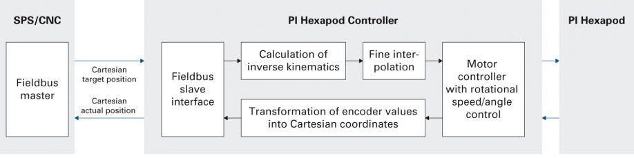
Figure 2: The control transmits and receives Cartesian coordinates on a regular basis. The typical cycle time is 1 millisecond (PI).

Communication via EtherCAT

The EtherCAT communication is based on the CANopen over EtherCAT (CoE) protocol and therefore offers the same communication mechanisms that are defined in the CANopen standard according to EN 50325-4.  The minimum permissible cycle time for the hexapod controller is one millisecond. The Object Dictionary, Process Data Object (PDO) Mapping, and Service Data Objects (SDO) are supported.

PDOs and SDOs have been defined according to drive profile CiA402 (IEC 61800-7-201/301, figure 3 and figure 4) in order to allow easy integration of the Cartesian axes of the hexapod within the PLC.

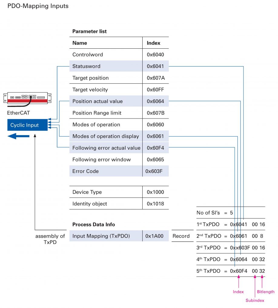
Figure 3: PDO Mapping Inputs for Hexapods (PI).

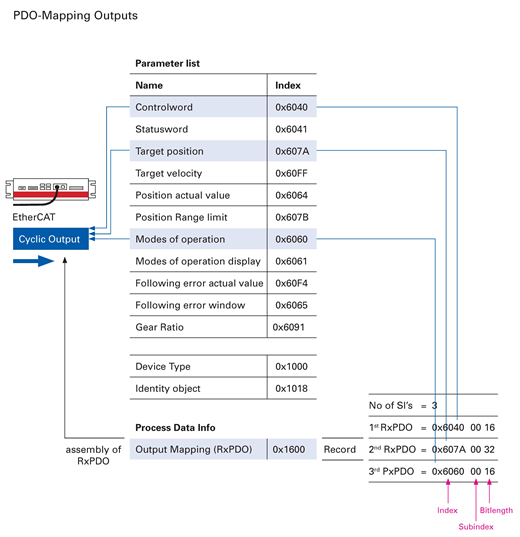
Figure 4: PDO Mapping Outputs for Hexapods (PI).

Coupling of the Axes

Since all drives act on the same platform, the statuses of the individual Cartesian axes are interdependent. Events that occur on one of the Cartesian axes affect the overall system. To counter this situation, each Cartesian axis is represented and treated as a separate axis in the PLC and the hexapod controller performs actions such as referencing or stopping the axis for all axes simultaneously. It is therefore sufficient to command such actions for only one Cartesian axis.

Error messages from one Cartesian axis are also mirrored on all other axes. However, in order not to intervene too comprehensively in the underlying standardized drive protocol, control and status words are maintained separately for each axis (figure 5).

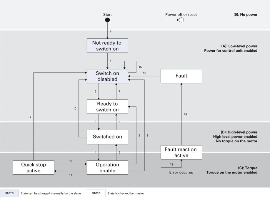
Figure 5: CiA402 Drive State Machine (PI).

Status transitions of an axis therefore have an influence on the entire hexapod system. The axis with the lowest status level determines the status of the system. To move the hexapod to a higher status level, all axes must have reached this level at a minimum. Conversely, it is sufficient to set an axis to a level lower than the overall system in order to also set it to the lower status level. Table 1 illustrates this relationship.

Table 1: The relationship between single-axis status and the status of the overall system according to the transitions shown in figure 5 (PI).

The status of the overall system can be queried at any time via object 0x5013:01. Table 2 shows the relationship between the displayed value and the status of the hexapod system.

Table 2: Relationship between the displayed value and the status of the hexapod system (PI).

The coupling of the axes also influences the activation of the various operating modes. This is controlled via the process data object Modes of Operation (0x6060), and only the first axis (X-axis) is taken into account. In all other axes, this object has no function. The operating mode in which the hexapod system is located is displayed in the process data object Modes of Operation Display (0x6061). The current value is mirrored to the respective objects of all axes.

There is support for operating modes Cyclic Synchronous Position Mode (CSP) and Homing as defined in CiA402.

Cyclic Synchronous Position Mode (CSP)

CSP mode is used to position the hexapod. The EtherCAT master specifies the target Cartesian positions for the axes cyclically and receives the actual Cartesian positions (figure 6).

When commanding the hexapod, note that the maximum vector velocity of the hexapod depends on the maximum possible velocity and acceleration of the individual struts. Depending on the angle of the hexapod platform and the commanded Cartesian target position, the hexapod achieves different maximum vector velocities.

If the maximum values of the hexapod are used in the PLC when configuring the Cartesian axes, the actual hexapod velocity will deviate from the velocity calculated in the PLC, and the greater the distance to be travelled, the greater the deviation. This can

lead to tracking errors and make control more difficult. One way of avoiding large tracking errors is to reduce the target velocity and acceleration in the PLC for combined movements of the Cartesian axes.

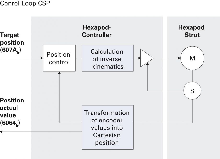
Figure 6: Servo Loop of the Cyclic Synchronous Positioning Mode (CSP) (PI).

If the maximum possible vector velocity of the hexapod is even exceeded when the target positions are specified, the stop mechanism integrated in the hexapod controller automatically takes effect. This puts the hexapod controller into an error state and brakes the system to a standstill with the maximum possible acceleration. The integrated interpolation mechanism ensures that the hexapod is kept on the planned path.

Range of Motion and Velocities

Various service data objects are available in order to avoid exceeding the vector velocity and to provide the user with the best possible support in trajectory planning.

Objects 0x5011 and 0x5012 can be used to determine the maximum possible travel range along a defined vector. The vector is defined in object 0x5011 and the calculation is started via a handshake bit in object 0x5010:03. The result of the calculation, the coordinates of the point at the boundary of the workspace along the given vector, is displayed in object 0x5012 (figure 7).

When querying the available travel range, the controller simultaneously calculates the maximum possible velocities and accelerations, distinguishing between translational and rotational components. Since the maximum possible velocities and accelerations vary

across the workspace, only values for the point at which the hexapod was located when the query was started are determined. The values for the velocities and accelerations are displayed in object 0x5014.

Regardless of vector velocity and acceleration, it is recommended that you also configure the values for the maximum and reference velocities and accelerations for the axes in the PLC. The velocities can be taken from the hexapod data sheet.

The acceleration values for the translation axes can be read out directly via service parameter 0x19001502 using PI software PIMikroMove or PITerminal. This can be done during initial commissioning, for example.

For the rotational axes, the maximum acceleration can be determined by transferring the ratio for linear axes.

Example: In the case of an H-820.D2, the maximum velocity is 20 mm/s for the translation axes and 11 °/s (200 mrad/s) for the rotational axes. The acceleration for the translation axis is 80 mm/s². This results in a rotational acceleration of

11 * 80 / 20 = 44 °/s².

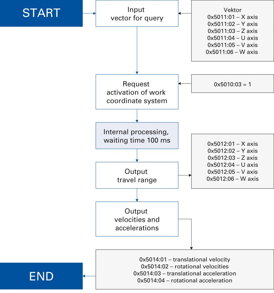
Figure 7: Procedure for Querying Travel Range and Velocities (PI).

Using Different Coordinate Systems

The intelligent hexapod controller allows the user to freely define and select reference coordinate systems for movement in space, and thus, to control the movement of the hexapod for the respective application in the best possible way.

A Work coordinate system and a Tool coordinate system are available to the user via the EtherCAT interface. For configuration of the coordinate systems, it is assumed that the Tool coordinate system moves in the Work coordinate system. A description is included in the corresponding user documentation.

Object 0x5000 is available to the user for configuration of the Work coordinate system. The sub-indices correspond to the coordinates of the individual Cartesian axes. The Tool coordinate system can also be configured via object 0x5001. All values must be specified in micrometers or thousandths of a degree.

After configuration, the coordinate systems must be activated. This is implemented via object 0x5010. The two coordinate systems are activated independently of each other via sub-index 1 for the Work coordinate system and sub-index for the Tool coordinate system. The activation of the coordinate systems and the associated recalculations of the kinematic transformations take about 100 milliseconds (figure 8).

During activation of coordinate systems, the actual position of the hexapod transmitted to the PLC will change. To prevent an unforeseen reaction from the PLC, the hexapod controller must therefore be set to Mode of Operation 0 to activate a coordinate system. In this mode, no new target positions of the PLC are processed and the Following Error transmitted to the PLC is set to value 0 for all axes. After successful activation of the coordinate systems, the target position must then be set equal to the current position within the PLC. Afterwards, it is possible to change to Mode of Operation = 8 and movements can be commanded in the new coordinate system configuration.

A change in the coordinate system configuration can affect the available range of motion and velocities. Therefore, the parameterization of the individual movements must also be adapted.

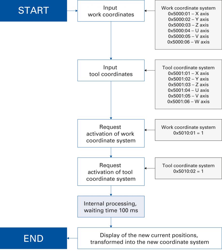
Figure 8: Configuration Procedure for Coordinate Systems (PI).

Additional Functions

Referencing

The Homing operating mode is used to perform a referencing run to the motor axis zero points that define the Cartesian zero point of the hexapod platform.

Since the PI portfolio includes both hexapods with absolute measuring sensors and hexapods with incremental measuring systems, all information regarding the referencing method and zero points is only used within the hexapod controller to calculate an absolute actual position for the PLC. Therefore, referencing is always performed as drive-controlled Homing. The necessary parameters for configuration of the referencing run are already stored in the hexapod controller. The PLC only has to start and stop the

referencing run process. The start takes place by changing the Mode of Operation and setting bit 4 in the Controlword of the X-axis. The current status of the referencing run is then displayed in the Statusword of the X-axis.

Dead-Time Compensation

The various mechanisms that ensure that the hexapod moves exactly on the path planned by the user require computing time. However, this so-called dead time can be compensated for on many controllers. The dead time is composed of time for communication and time for interpolation. Therefore, the dead time for the hexapod controller depends on the set EtherCAT cycle time. The dead time can be calculated as follows for any cycle time:

𝑡𝑑𝑒𝑎𝑑 = 4 ∗ 𝑡𝑐𝑦𝑐𝑙𝑒 + 5 ∗ 𝑡𝑖𝑛𝑡𝑒𝑟𝑝𝑜𝑙𝑎𝑡𝑖𝑜𝑛 𝑏𝑢𝑓𝑓𝑒𝑟

𝑡_{𝑑𝑒𝑎𝑑}:  Dead time

𝑡_{𝑐𝑦𝑐𝑙𝑒}:  Cycle time

𝑡_{𝑖𝑛𝑡𝑒𝑟𝑝𝑜𝑙𝑎𝑡𝑖𝑜𝑛 𝑏𝑢𝑓𝑓𝑒𝑟}: 𝐼𝑛𝑡𝑒𝑟𝑝𝑜𝑙𝑎𝑡𝑖𝑜𝑛 b𝑢𝑓𝑓𝑒𝑟

− time = 2 𝑚𝑠

A cycle time of one millisecond results in a dead time of 14 milliseconds. In addition to calculation of this time, empirical optimization is recommended.

Quick-Stop Function for Emergency Stop

If a quick stop is requested during a movement, such as in the context of an emergency stop of the system, the hexapod is brought to a standstill with the maximum possible deceleration. The integrated path interpolation ensures that the hexapod continues to move on the previously requested path.

Command via GCS

The initial commissioning of the hexapod system should always be carried out via the PI software. All required parameters are also queried and can then be transferred to the PLC. Ethernet and RS-232 interfaces are available on the hexapod controller.

Even with the EtherCAT interface activated, it is possible to send GCS commands at any time via the Ethernet and RS-232 interfaces on the hexapod controller. However, as soon as the individual axes are set to the status Operation enabled by the PLC, all GCS commands that command or stop a movement, as well as commands that result in a change of the displayed current position, are blocked.

Details on commanding with PI’s own GCS command set can be found in the relevant manuals and user documentation.

*EtherCAT® is a registered trademark and patented technology licensed from Beckhoff Automation GmbH, Germany.

About the Author

Dr. Steffen Schreiber is Senior Expert on Hexapod Development at PI.  He has been working for many years with fieldbus systems, especially EtherCAT. He is driven in particular by the challenge of optimally integrating parallel-kinematic systems, such as hexapods.

About Physik Instrumente L.P.

Physik Instrumente L.P. (PI) is a leading manufacturer of nanopositioning, linear actuators and precision motion-control equipment for photonics, nanotechnology, semiconductor and life science applications.   PI has been developing and manufacturing standard and custom precision products with piezoelectric and electromagnetic drives for over 50 years.  The company has been ISO 9001 certified since 1994, and with more than 350 granted and pending patents, provides innovative, high-quality solutions for OEM and research.  PI has a worldwide presence with 10 subsidiaries and over 1,300 staff.

For more information please contact Stefan Vorndran, VP Marketing for Physik Instrumente L.P.; 16 Albert St., Auburn, MA 01501; Phone 508-832-3456, Fax 508-832-0506; email stefanv@pi-usa.us; www.pi-usa.us.